SQL Query Performance: 5 Fixes That Actually Work
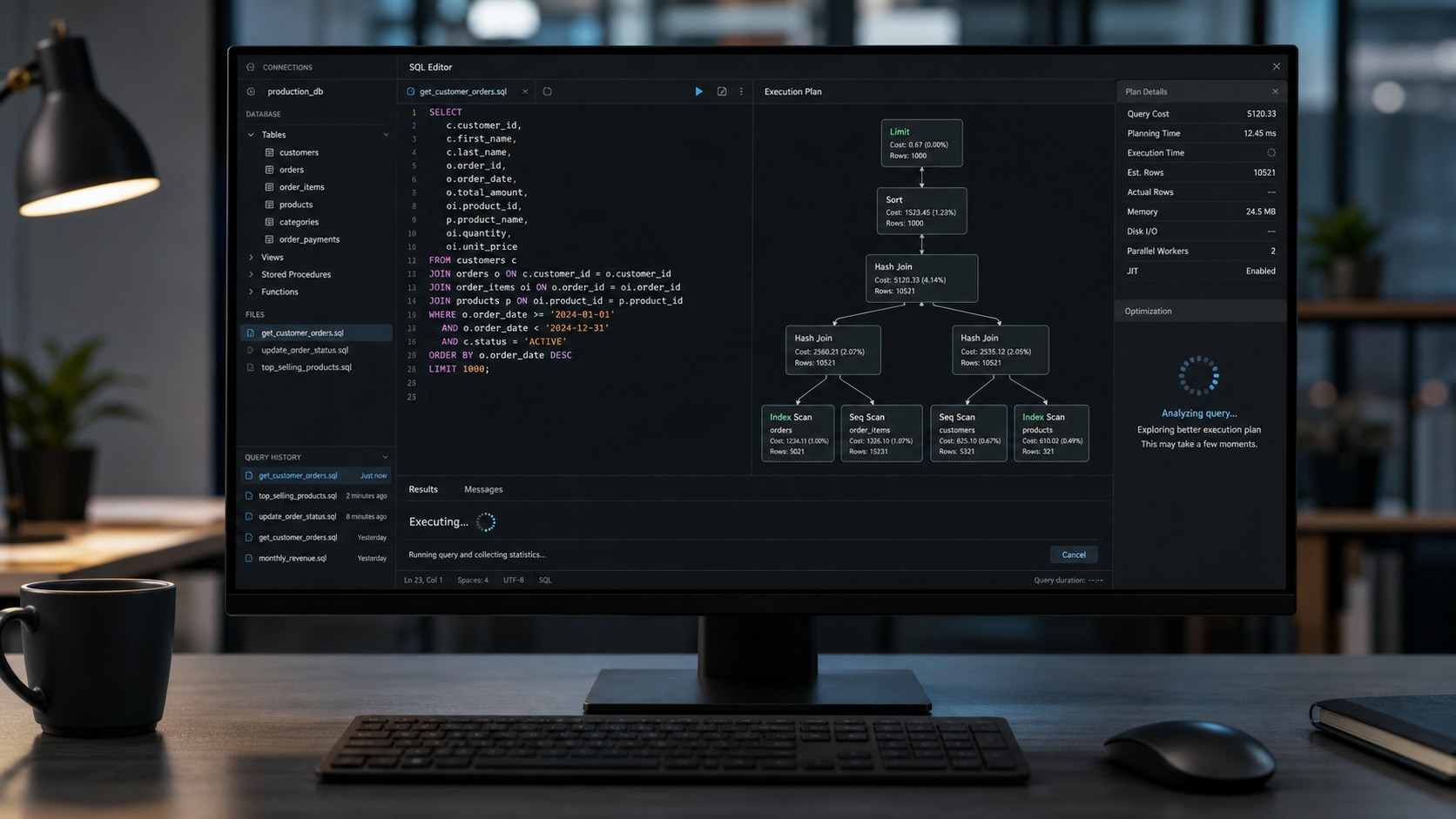
Slow queries are the most common thing that makes a data engineer look bad in a meeting. Someone runs a dashboard, the spinner turns for 20 seconds, and the Slack message hits your DMs before the query finishes. This guide covers the five fixes that resolve 80% of production slowdowns—each with a concrete example you can run against your own warehouse.
Fix 1: Missing (or wrong) indexes
An index is a sorted lookup structure. Without one on a JOIN or WHERE column, the database scans every row in the table. With one, it jumps directly to the matching rows.
Before (full table scan):
SELECT o.order_id, c.name
FROM orders o
JOIN customers c ON o.customer_id = c.id
WHERE o.order_date >= '2026-01-01';

-- Seq Scan on orders  (cost=0.00..48500.00 rows=120000 width=40)
--   Filter: (order_date >= '2026-01-01')
After (indexed lookup):
CREATE INDEX idx_orders_customer_date ON orders(customer_id, order_date);

-- Index Scan using idx_orders_customer_date on orders
--   (cost=0.42..8500.00 rows=120000 width=40)
The index cut the cost from 48,500 to 8,500—roughly a 6x improvement, and the gap grows with table size. The compound index on (customer_id, order_date) serves both the JOIN and the WHERE in one structure.
Rule: Index every column used in JOINs and WHERE clauses on large tables. Use compound indexes when a query filters on multiple columns. But don’t index everything: each index adds write overhead. For a table that’s read 100x more than written, index freely. For a high-write table (event logs, clickstreams), be selective.
Fix 2: SELECT * on wide tables
SELECT * fetches every column, including large text fields, JSON blobs, and geo columns you don’t need. In a warehouse with columnar storage (BigQuery, Snowflake, Redshift), the cost difference is proportional: reading three columns is often 10–20x cheaper than reading forty.
Before:
SELECT *
FROM analytics_events
WHERE event_date = '2026-07-06';
-- Scanned: 42 GB (all 68 columns)
After:
SELECT event_id, event_type, user_id, event_timestamp
FROM analytics_events
WHERE event_date = '2026-07-06';
-- Scanned: 2.1 GB (4 columns)
The fix is mechanical: list the columns you actually need. If you’re building a dashboard query, only select the columns that appear in the chart. Your warehouse bill will thank you.
Fix 3: Nested subqueries vs CTEs vs JOINs
A subquery inside a WHERE clause often runs once per outer row, turning an O(n) scan into O(n²). A CTE or a JOIN gives the optimizer room to pick a better plan.
Before (correlated subquery — runs per row):
SELECT user_id, order_total
FROM orders o
WHERE order_total > (
  SELECT AVG(order_total)
  FROM orders
  WHERE user_id = o.user_id
);
After (CTE + JOIN — runs once):
WITH user_avg AS (
  SELECT user_id, AVG(order_total) AS avg_total
  FROM orders
  GROUP BY user_id
)
SELECT o.user_id, o.order_total
FROM orders o
JOIN user_avg u ON o.user_id = u.user_id
WHERE o.order_total > u.avg_total;
In modern optimisers (Postgres ≥ 12, recent MySQL), simple subqueries are often rewritten into JOINs automatically. But correlated subqueries—those referencing a column from the outer query—rarely get rewritten. The CTE pattern makes the intent explicit and nearly always beats the correlated version.
Fix 4: Implicit type casting in JOINs
When you JOIN on columns of different types—say a VARCHAR customer_id in one table and an INTEGER in another—the database silently casts one side for every comparison. This drops the index and triggers a full scan.
Before (implicit cast kills the index):
-- orders.customer_id is INTEGER, users.id is VARCHAR
SELECT *
FROM orders o
JOIN users u ON o.customer_id = u.id;
-- Seq Scan on users: implicit cast on every row
After (explicit cast, or fix the schema):
-- Option A: cast the indexed side (cheap, one-time)
SELECT *
FROM orders o
JOIN users u ON CAST(o.customer_id AS VARCHAR) = u.id;

-- Option B (better): fix the column type in the source table
ALTER TABLE users ALTER COLUMN id TYPE INTEGER USING id::INTEGER;
How to spot it: Look at your EXPLAIN output for rows where the database says “Filter” on a JOIN column instead of “Index Scan.” Check the column types in your schema with SELECT column_name, data_type FROM information_schema.columns WHERE table_name = 'orders';
Fix 5: Unanchored JOINs (cartesian products)
An unanchored JOIN—also called a cross join or cartesian product—mates every row in the left table with every row in the right. Two tables of 10,000 rows each produce 100 million intermediate rows. This is the fastest way to bring a warehouse to its knees.
Before (accidental cross join):
SELECT o.order_id, p.product_name
FROM orders o, products p
WHERE o.order_date = '2026-07-06';
-- 10,000 orders x 5,000 products = 50 million rows (then filtered)
After (anchored JOIN):
SELECT o.order_id, p.product_name
FROM orders o
JOIN order_items oi ON o.id = oi.order_id
JOIN products p ON oi.product_id = p.id
WHERE o.order_date = '2026-07-06';
-- Each JOIN has a real condition; row count stays sane
The comma-style FROM a, b syntax is the most common culprit—it’s easy to forget the WHERE clause that anchors it. Prefer explicit JOIN ... ON syntax: it makes the anchor condition mandatory and obvious to anyone reading the query.
FAQ
How do I read an EXPLAIN plan?
Start from the innermost node and read outward. Each row is an operation: a Seq Scan reads the whole table (bad for large tables), an Index Scan uses an index (good), a Nested Loop JOINs rows one-by-one (fine for small sets, expensive for large), a Hash Join builds an in-memory hash table (good for medium-to-large). The cost=x..y numbers are arbitrary units: lower is faster. Focus on the ratio, not the absolute number.
Should I use a covering index?
A covering index includes all columns the query needs, so the database never touches the main table. For high-frequency dashboard queries that fetch the same 3–5 columns, a covering index can be 10–100x faster. The trade-off is more storage and slower writes. Use them for read-heavy, narrow queries on large tables.
When do indexes hurt performance?
Every INSERT, UPDATE, and DELETE on an indexed column must also update the index. On a table getting thousands of writes per second, too many indexes slow ingestion to a crawl. Profile your read/write ratio: if writes dominate, be conservative with indexes.
Does query optimization differ by warehouse?
Yes. Row-store databases (Postgres, MySQL) rely heavily on indexes. Column-store warehouses (BigQuery, Snowflake, Redshift) don’t use traditional indexes—they optimize through partitioning, clustering keys, and minimizing bytes scanned. The SELECT * fix is far more important on columnar warehouses than the index fixes, which mostly apply to row-store systems.
These five fixes cover the bulk of what makes a slow query slow. Internalize them, and the next Slack DM about a slow dashboard will have an answer in under two minutes. For a deeper look at how data flows through the systems you’re querying, start with the star schema guide and the modern data stack overview. For more advanced SQL patterns, the SQL window functions guide covers the next level.
Last updated: July 10, 2026


Comments
Post a Comment